HQC-Bend: Hybrid Quantum-Classical Multi-cuts Benders' Decomposition

01 · Motivation

(Mixed-)integer linear programs are everywhere, and they are hard

Many planning and operations problems mix yes/no decisions (open a route, start a generator, switch on a chiller) with continuous quantities (flows, power, temperatures). That mix is a (mixed-)integer linear program, or (M)ILP.

Network problemsBalancing production and demand across plants, warehouses and retailers.
Route planningChoosing vehicle routes that cut transport cost and distance.
Data center energy managementScheduling batteries, chillers and cooling towers under thermal limits.
Unit commitmentDeciding which power generators run in each hour.

~10% forecast annual growth in US data center power demand through 2030 (McKinsey). Faster solvers for these energy problems are needed.

Why it is hard

\begin{aligned} \max_{\mathbf{x},\mathbf{y}}\ & \mathbf{c}^{\intercal}\mathbf{x} + \mathbf{h}^{\intercal}\mathbf{y} \\ \text{s.t. }\ & \mathbf{T}\mathbf{x} \leqq \mathbf{p} \\ & \mathbf{A}\mathbf{x} + \mathbf{G}\mathbf{y} \leqq \mathbf{b} \\ & \mathbf{x} \in \mathbb{Z}^{n},\ \mathbf{y} \in \mathbb{R}^{m} \end{aligned}

(M)ILP is NP-hard: unless P = NP, no algorithm solves every instance in polynomial time.

PGraph connectivity
NPFactoring
NP-completeGraph 3-coloring
NP-hard(M)ILP, halting problem

The classical toolbox includes enumerative methods, branch and bound, and cutting planes. All of them run on CPUs.

02 · Quantum vs classical

CPU? QPU? Use both.

Each processor is strong where the other is weak. HQC-Bend gives each one the part of the problem it is suited to.

	Advantages	Disadvantages
CPU Central Processing Unit	Versatile Efficient for classical algorithms	Limited parallelism Slower for certain tasks
QPU Quantum Processing Unit	Quantum parallelism Quantum tunneling, which escapes local minima Exponential speedup on some problems*	Limited to specialized cases High error rates in the NISQ (noisy intermediate-scale quantum) era

Activate the spread

Superposition spans a vast space of candidate solutions at once.

Encode the problem

The optimization problem is embedded into the quantum system's energy landscape.

Unleash the power

The system settles into low-energy states, which are read back as classical solutions.

QPU

The master problem is purely binary, which is the form annealers natively solve (QUBO).

CPU

The subproblems are continuous linear programs, which classical solvers handle fast and in parallel.

03 · How it works

One class, three stages, one loop

HQC-Bend decomposes the target model into a binary master problem (MAP) and continuous subproblems (SUB), then iterates between them.

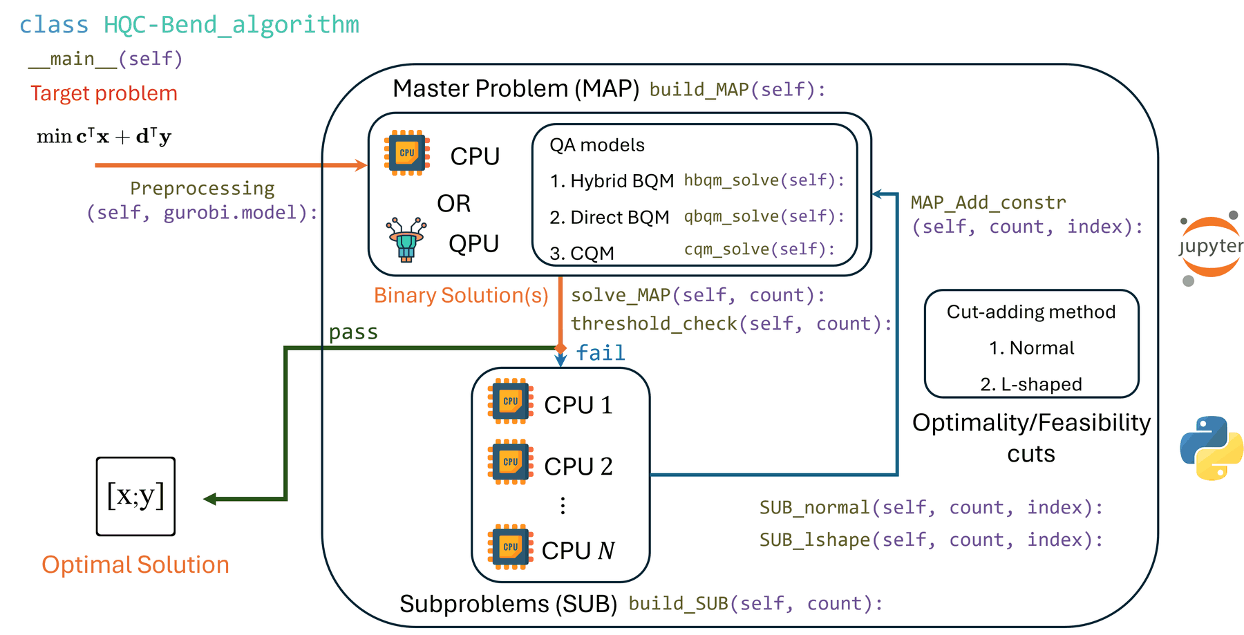
Architecture of the HQC-Bend algorithm: the target Gurobi model is preprocessed (1), the master problem is solved on a CPU or a QPU using Hybrid BQM, Direct BQM or CQM (2), and if the threshold check fails the binary solutions are sent to subproblems solved on CPUs 1 to N with the normal or L-shaped scheme (3), which return optimality and feasibility cuts to the master problem. When the check passes, the optimal solution [x; y] is returned. — Logic flow of the algorithm class. The numbered stages are described below.

Preprocessing

Reads your gurobipy model, separates binary \mathbf{x} from continuous \mathbf{y}, and extracts the matrices.

\mathbf{c},\mathbf{H},\mathbf{e} go to the MAP. \mathbf{d},\mathbf{A},\mathbf{G},\mathbf{b} go to the SUBs.

Master problem

Solved on a CPU (Gurobi) or a QPU (D-Wave CQM/BQM) or by a local quantum-inspired sampler. It returns one or more binary candidates \mathbf{x}^{*}.

A threshold check on the λ bounds decides whether to stop.

Subproblems & cuts

For each candidate, the subproblems run on CPUs 1…N with the normal, L-shaped or Benders dual scheme and return optimality or feasibility cuts to the MAP.

The loop repeats until the gap closes or max_steps is reached.

Target model

\begin{aligned} \min\ & \mathbf{c}^{\intercal}\mathbf{x} + \mathbf{d}^{\intercal}\mathbf{y} \\ \text{s.t. }\ & \mathbf{A}\mathbf{x} + \mathbf{G}\mathbf{y} \leqq \mathbf{b}, \\ & \mathbf{H}\mathbf{x} \leqq \mathbf{e}, \\ & \mathbf{x} \in \mathbb{B}^{n},\ \mathbf{y} \in \mathbb{R}^{m}. \end{aligned}

Master problem (MAP)

\begin{aligned} \min_{\mathbf{x},\lambda,\mathbf{z}}\ & \mathbf{c}^{\intercal}\mathbf{x} + \lambda \\ \text{s.t. }\ & \mathbf{H}\mathbf{x} \leqq \mathbf{e}, \\ & f(\lambda,\mathbf{x}) \le 0 \quad \text{(optimality cuts)}, \\ & f(\mathbf{x}) \le 0 \quad \text{(feasibility cuts)}, \\ & \lambda = g(\mathbf{z}) \quad \text{(discretization)}, \\ & \mathbf{x} \in \mathbb{B}^{n},\ \lambda \in \mathbb{Q},\ \mathbf{z} \in \mathbb{B}^{l}. \end{aligned}

Key features

Hybrid quantum-classical computing. QPU for the binary master problem, CPUs for the continuous subproblems.
Modular structure. Preprocessing, master solvers and cut schemes are separate pieces you can extend.
Gurobi and Python native. Input is a plain gurobipy model. Runs as a script or in Jupyter Notebook.
Parallel subproblems. Multiple binary candidates are evaluated on CPU clusters.
Stronger cuts. Benders dual decomposition lifts cuts on the LP relaxation of the master before the binary loop starts.
Several quantum backends. D-Wave BQM and CQM solvers, plus the OpenJij and simulated-bifurcation samplers.

04 · Master-problem solvers

From binary master problem to QUBO

The master problem is binary because λ is discretized into bits (see Configure). Each quantum mode encodes the objective and constraints as a QUBO, with each constraint added as a penalty term:

f(\mathbf{x}) \;\longrightarrow\; \text{QUBO} \;=\; \text{QUBO}_{\text{obj}} \;+\; \sum_{c \,\in\, \text{constraints}} P_c \cdot g(\text{constraint}_c)

Here P_c is the penalty coefficient of constraint c and g(\cdot) is its encoded penalty.

CPUHybrid_mode: false

Gurobi

Classical baseline. The MAP is solved exactly with Gurobi, one cut per iteration.

CPU + QPU"cqm"

Constrained Quadratic Model

D-Wave Leap hybrid CQM solver. Constraints are passed natively instead of as penalties.

CPU + QPU"bqm_hybrid"

Hybrid BQM

D-Wave Leap hybrid sampler. Classical and quantum modules work together for balanced performance.

QPU"bqm_quantum"

Direct BQM

Pure quantum annealing on a D-Wave QPU through an embedding composite.

Local"openjij"

OpenJij

Quantum-inspired annealing on your own machine. No cloud token needed.

Local"bifurcation"

Simulated bifurcation

Quantum-inspired Ising solver built on PyTorch, run by HQC-Bend on an NVIDIA GPU. GPU install guide

Inside D-Wave's Hybrid Solver Service

The hybrid modes run on D-Wave's Hybrid Solver Service, which pairs a Classical Heuristic module (CH) with a Quantum Module (QM) in several parallel threads. Together they return one or more high-quality candidate solutions. HQC-Bend can turn each candidate into its own cut (multi-cuts).

Scheme after Osaba, Villar-Rodríguez, Gomez-Tejedor and Oregi, “Hybrid quantum solvers in production: how to succeed in the NISQ era?”, IDEAL 2024, pp. 423–434.

05 · Cut-adding schemes

Three ways to cut: normal, L‑shaped and Benders dual

Given a binary candidate \mathbf{x}^{*} from the MAP, the subproblem produces a dual solution \mathbf{w}^{*}, which becomes one of two cuts:

Optimality cut

(\mathbf{b} - \mathbf{A}\mathbf{x})^{\intercal}\mathbf{w}^{*} \le \lambda

Feasibility cut

(\mathbf{b} - \mathbf{A}\mathbf{x})^{\intercal}\mathbf{w}^{*} \le 0

Primal subproblem (PSUB)

\begin{aligned} \lambda = \min_{\mathbf{y}}\ & \mathbf{d}^{\intercal}\mathbf{y} \\ \text{s.t. }\ & \mathbf{G}_1\mathbf{y} = \mathbf{b}_1 - \mathbf{A}_1\mathbf{x}^{*} \quad (1) \\ & \mathbf{G}_2\mathbf{y} \ge \mathbf{b}_2 - \mathbf{A}_2\mathbf{x}^{*} \quad (2) \\ & \mathbf{y} \ge \mathbf{0} \end{aligned}

Dual subproblem (DSUB)

\begin{aligned} \max_{\mathbf{w}}\ & \left(\begin{bmatrix}\mathbf{b}_1\\ \mathbf{b}_2\end{bmatrix} - \begin{bmatrix}\mathbf{A}_1\\ \mathbf{A}_2\end{bmatrix}\mathbf{x}^{*}\right)^{\intercal} \begin{bmatrix}\mathbf{w}_{(1)}\\ \mathbf{w}_{(2)}\end{bmatrix} \\ \text{s.t. }\ & \begin{bmatrix}\mathbf{G}_1\\ \mathbf{G}_2\end{bmatrix}^{\intercal} \begin{bmatrix}\mathbf{w}_{(1)}\\ \mathbf{w}_{(2)}\end{bmatrix} \le \mathbf{d} \\ & \mathbf{w}_{(1)} \in \mathbb{R},\ \mathbf{w}_{(2)} \in \mathbb{R}^{+} \end{aligned}

Solve the dual subproblem DSUB at the current \mathbf{x}^{*}.
If DSUB has an optimal solution \mathbf{w}^{*}, add an optimality cut.
Otherwise the subproblem is infeasible for this \mathbf{x}^{*}: add a feasibility cut.

Benders dual decomposition (Rahmaniani et al., Operations Research, 2020) gives the subproblem binary copies \mathbf{z} of the master variables and prices the copy constraint \mathbf{z} = \mathbf{x} into the objective with multipliers \boldsymbol{\pi}.

Lagrangian subproblem

\begin{aligned} L(\boldsymbol{\pi}) = \min_{\mathbf{y},\mathbf{z}}\ & \mathbf{d}^{\intercal}\mathbf{y} - \boldsymbol{\pi}^{\intercal}\mathbf{z} \\ \text{s.t. }\ & \mathbf{A}\mathbf{z} + \mathbf{G}\mathbf{y} \leqq \mathbf{b}, \\ & \mathbf{H}\mathbf{z} \leqq \mathbf{e}, \\ & \mathbf{y} \ge \mathbf{0},\ \mathbf{z} \in \mathbb{B}^{n} \end{aligned}

BDD cuts

\begin{aligned} \lambda \ &\ge\ L(\boldsymbol{\pi}) + \boldsymbol{\pi}^{\intercal}\mathbf{x} \quad \text{(optimality)} \\ 0 \ &\ge\ F(\boldsymbol{\beta}) + \boldsymbol{\beta}^{\intercal}\mathbf{x} \quad \text{(feasibility)} \end{aligned}

F(\boldsymbol{\beta}) is the same problem with a penalized slack \mathbf{s} on every row and objective \mathbf{1}^{\intercal}\mathbf{s} - \boldsymbol{\beta}^{\intercal}\mathbf{z}. With \boldsymbol{\pi} fixed to the LP multipliers the cut keeps the classical slope and gets a higher right-hand side (strengthened cut); optimizing \boldsymbol{\pi} gives a Lagrangian cut.

Phase 1 · classical. Solve the LP relaxation of the master and add classical cuts at its fractional points.
Phase 2 · strengthened. Keep the LP multipliers and lift each cut by solving the MILP above (eq. 9–10, 12–13).
Phase 3 · Lagrangian. Update \boldsymbol{\pi} with a regularized cutting-plane step (eq. 15–16) to push the cut further.

At a binary master point these cuts equal the classical ones, so BDD runs at the LP root before the first master solve and the main loop then adds L-shaped cuts. The subproblem MILPs also return feasible solutions; the best one is saved as an incumbent in data_output/bdd_info.json.

Multi-cuts

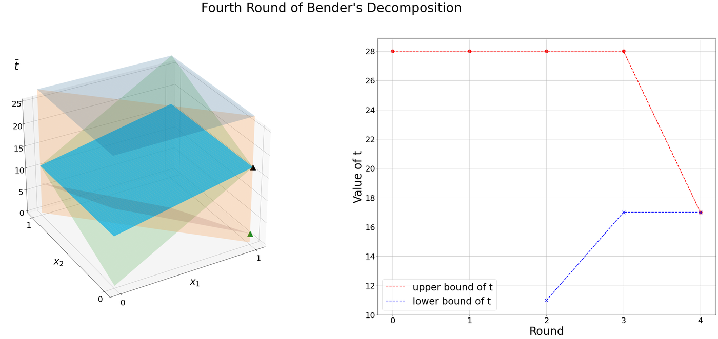
A quantum sampler returns a whole distribution of low-energy binary states, not just one. With Mcut_flag: true, HQC-Bend takes the best Cutnums candidates, solves their subproblems in parallel on CPUs, and adds one cut per candidate in a single iteration. More cuts per round tighten the bounds on λ faster.

Each cut is a plane that bounds λ from below. Rounds continue until the upper and lower bounds of λ are within threshold.gap.

Left: 3D plot of cutting planes over binary variables x1 and x2 bounding t from below. Right: upper bound of t stays at 28 for three rounds then drops to 17 while the lower bound rises from 11 to 17, meeting at round 4. — Fourth round of Benders' decomposition. Left: the accumulated cutting planes. Right: the upper and lower bounds of λ (shown as t) meet at round 4.

06 · Configuration

Change the method, not the code

A JSON file controls the solver backend, the cut scheme, the precision of λ and the stopping rule. mode="manual" reads config.json and mode="default" reads config_default.json. Users can change the mathematical method even with little background in the field.

Connection variable λ

Non-negative bits Decimal bits Negative bits

Algorithm

Sub-method Max steps Stopping rule Gap

Hybrid_mode (quantum master problem) debug_mode (export LP files)

Benders dual decomposition (bdd)

Root iterations Lagrangian iterations MIP gap Time limit (s)

Quantum backend

Mode num_of_read Cutnums DWave_token

Mcut_flag (multi-cuts per iteration)

config.json

Save it as config.json next to HQCMCBD.py and run with mode="manual".

All configuration keywords

Keyword	Meaning	Values
`lambda_var`	Connection variable λ between the MAP and the SUBs, written as \lambda = \lambda_{+}^{\mathbb{Z}} + \lambda_{+}^{\mathbb{Q}\setminus\mathbb{Z}} - \lambda_{-}^{\mathbb{Z}}	object
`nonneg_bits_length`	Bits for the non-negative integer part \lambda_{+}^{\mathbb{Z}}	positive integer
`decimal_bits_length`	Bits for the positive fractional part \lambda_{+}^{\mathbb{Q}\setminus\mathbb{Z}}	positive integer
`negative_bits_length`	Bits for the negative integer part \lambda_{-}^{\mathbb{Z}}	positive integer
`submethod`	Method for solving the subproblems	`normal`, `l_shape`, `bdd`
`bdd.root_iterations`	Maximum LP iterations of the BDD root phase; `0` behaves like `l_shape`	non-negative integer
`bdd.lagrangian_iterations`	Maximum multiplier updates per Lagrangian cut; `0` stops after strengthened cuts	non-negative integer
`bdd.mip_gap`	Gurobi `MIPGap` for the BDD subproblems	non-negative number
`bdd.time_limit`	Gurobi time limit in seconds for each BDD subproblem	positive number or `null`
`debug_mode`	Export LP files of the master problem and subproblems	`true`, `false`
`Hybrid_mode`	Solve the master problem with a quantum or quantum-inspired backend (Q+C) instead of Gurobi (C+C)	`true`, `false`
`dwave.mode`	How the MAP is encoded for the quantum solver	`cqm`, `bqm_hybrid`, `bqm_quantum`, `openjij`, `bifurcation`
`dwave.DWave_token`	D-Wave Leap API token. Placeholder values fall back to the `DWAVE_API_TOKEN` environment variable	string
`dwave.Mcut_flag`	Add multiple cuts per iteration (otherwise one)	`true`, `false`
`dwave.Cutnums`	Number of cuts per iteration when `Mcut_flag` is true	positive integer
`dwave.num_of_read`	Number of samples to read from the quantum solver	positive integer
`threshold.type`	Which gap the stopping rule checks: absolute \|\bar\lambda - \underline\lambda\| or relative 100\cdot\|\bar\lambda - \underline\lambda\| / \|\bar\lambda\| (in percent)	`absolute`, `relative`
`threshold.gap`	The run stops once the chosen gap drops below this value ε	positive number
`max_steps`	The algorithm stops after this many iterations	positive integer

07 · Quick start

From a Gurobi model to a hybrid solve

1
Install

Requires Python 3.8+ and Gurobi 9.1.2+ with a valid license. HQCMCBD.py imports every backend when it loads, so install all of them even if you plan to use one mode.
```
git clone https://github.com/djzts/HQCMCBD-API.git
cd HQCMCBD-API
pip install gurobipy numpy dimod dwave-system openjij torch simulated-bifurcation
```
For the D-Wave modes (cqm, bqm_hybrid, bqm_quantum), set DWAVE_API_TOKEN in your environment rather than committing a token to the config file.
GPU-accelerated simulated bifurcation ("bifurcation")

The bifurcation backend calls simulated_bifurcation.minimize(..., device="cuda"), so it needs an NVIDIA GPU whose driver supports CUDA 11.8. The GPU_acced_Q installation guide covers the setup step by step: Python 3.10 (a conda environment is recommended), PyTorch 2.6.0 built for CUDA 11.8, and simulated-bifurcation 1.2.0. In short, run these after the install command above so the GPU build of PyTorch is not replaced:
```
pip install torch==2.6.0 torchvision==0.21.0 torchaudio==2.6.0 --index-url https://download.pytorch.org/whl/cu118
pip install simulated-bifurcation==1.2.0
python -c "import torch, simulated_bifurcation as sb; print(torch.__version__, torch.cuda.is_available())"
```
The last command should print 2.6.0+cu118 True. PyTorch's cu118 wheels include the CUDA runtime, so no separate CUDA Toolkit is needed. If it prints False, see the guide's troubleshooting section.

Import

Python script

from HQCMCBD import HQCMCBD_algorithm

Jupyter Notebook

import warnings
warnings.filterwarnings("ignore")
%run HQCMCBD_notebook.ipynb

Build your model

Any gurobipy model with binary variables and non-negative continuous variables works. This is the example problem from the package (Example.ipynb).

import gurobipy as gp
from gurobipy import GRB
import numpy as np

A = np.array([[0, 0], [0, 0], [0, 0], [0, 0],
              [-1, -1], [-1, 0], [-1, 0], [0, -1], [0, -1]])
G = np.array([[1, 0, 1, 0], [1, 0, 0, 1], [0, 1, 1, 0], [0, 1, 0, 1],
              [0, 0, 0, 0], [1, 0, 0, 0], [0, 1, 0, 0], [0, 0, 1, 0], [0, 0, 0, 1]])
b = np.array([1, 1, 1, 1, -1, 0, 0, 0, 0])
c = np.hstack(np.array([-15.0, -10.0]))
h = np.hstack(np.array([8, 9, 5, 6]))

# Create a new Gurobi model
model = gp.Model("MILP")

# Add variables
x = model.addMVar(shape=len(c), vtype=GRB.BINARY, name="x")
y = model.addMVar(shape=len(h), vtype=GRB.CONTINUOUS, lb=0, name="y")
z = model.addVar(vtype=GRB.CONTINUOUS, lb=0, name="z")
p = model.addVar(vtype=GRB.BINARY, name="p")

# Objective and constraints
model.setObjective(c @ x + h @ y, GRB.MAXIMIZE)
model.addConstr(A @ x + G @ y <= b, name="constraints")
model.addConstr(z == 1, name="constraints_eq")
model.addConstr(p == 1, name="constraints_eq2")

model.optimize()

Maximization models are converted to minimization internally and reported back in the original sign convention.

Run it (two lines)

Your methods · config.json

solver = HQCMCBD_algorithm(model, mode="manual")
solver.run()

Defaults · config_default.json

solver = HQCMCBD_algorithm(model, mode="default")
solver.run()

Follow the convergence

Each round prints the objective value, the λ bounds, and the relative and absolute gaps. The run stops when the gap meets the threshold.

Output · Example-3bin-output.ipynb, manual mode (abridged)

Benders decomposition Round - 2
The 2-th Config file of quantum sampling is created successfully at .\data_output\Gurobi_info-round-2.json.
create optimality cut
Round 2:
    Current Objective value is 12.0;
    lambda_upper is 20.0;
    lambda_lower is 11.0;
    Relative gap is 81.818%.
    Absolute gap is 9.0
Benders decomposition Round - 3
create optimality cut
Round 3:
    Current Objective value is 6.0;
    lambda_upper is 19.0;
    lambda_lower is 17.0;
    Relative gap is 11.765%.
    Absolute gap is 2.0
Benders decomposition Round - 4
create optimality cut
Round 4:
    Current Objective value is 5.0;
    lambda_upper is 17.0;
    lambda_lower is 17.0;
    Relative gap is 0.0%.
    Absolute gap is 0.0
optimal found, it takes 4  Rounds.

data_output/Objective values, λ bounds, solver metadata and MAP solutions for every round.

LP_output/Gurobi LP exports of the MAP and subproblems when debug_mode is on.

LP_output_dwave/Artifacts from the quantum and quantum-inspired solvers.

08 · Results

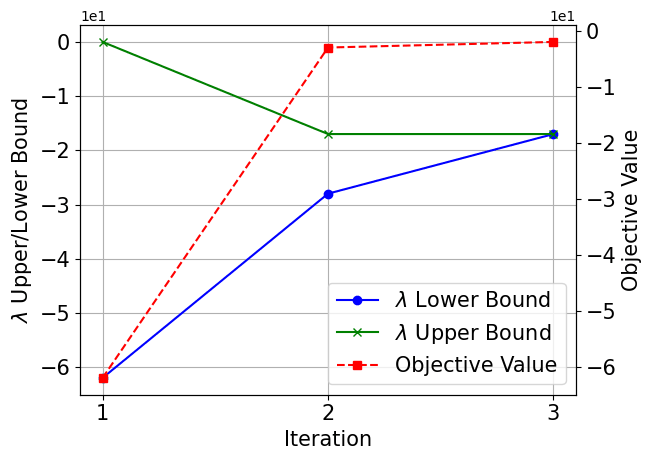
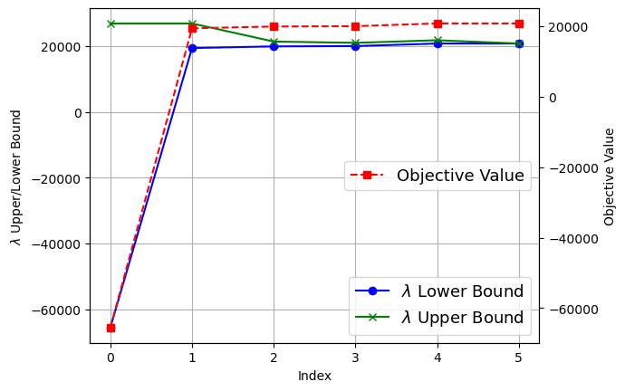
Bounds that close in a handful of rounds

Both plots track the lower and upper bounds of the connection variable λ and the objective value at each iteration.

Example problem: lambda lower bound rises from -62 to -17 and lambda upper bound falls from 0 to -17 over three iterations, while the objective value converges near -2. — **Example problem.** The quick-start model above. The λ bounds meet after three iterations.

Unit commitment problem: lambda bounds and objective jump from about -65,000 to about 20,000 after the first iteration and converge within five iterations. — **Unit commitment.** A classic power-system MILP. The objective and the bounds converge rapidly.

Example problem data

\mathbf{A}_2=\begin{bmatrix}0&0\\0&0\\0&0\\0&0\\-1&-1\\-1&0\\-1&0\\0&-1\\0&-1\end{bmatrix},\ \mathbf{G}_2=\begin{bmatrix}1&0&1&0\\1&0&0&1\\0&1&1&0\\0&1&0&1\\0&0&0&0\\1&0&0&0\\0&1&0&0\\0&0&1&0\\0&0&0&1\end{bmatrix},\ \mathbf{b}_2=\begin{bmatrix}1\\1\\1\\1\\-1\\0\\0\\0\\0\end{bmatrix}

\mathbf{d}^{\intercal}=\begin{bmatrix}8&9&5&6\end{bmatrix},\quad \mathbf{c}^{\intercal}=\begin{bmatrix}-15&-10\end{bmatrix}.

Takeaway

HQC-Bend is a Python package that solves complex (M)ILP problems with the HQC-Bend algorithm. It uses quantum computing for the optimization tasks it suits and classical solvers for the rest, giving an efficient and robust way to handle (M)ILP problems.

09 · Application

Data center energy management

The companion repository djzts/HQCMBD contains a data center model built for HQC-Bend. It is a natural fit: on/off decisions are binary and go to the quantum master problem, while power flows and temperatures are continuous and go to the CPU subproblems.

9server zones (3 × 3 grid)
150 kWhbattery, 60 / 90 kW charge / discharge limits
15–24 °Callowed zone temperature
2.5 kW/m²IT and server load density

The decisions

binary Battery charge / discharge status u^{\text{chr}}_t, u^{\text{dis}}_t
binary Chiller and cooling-tower on/off x^{\text{chiller}}_{j,t}, x^{\text{tower}}_{j,t}
continuous Battery power p^{\text{chr}}_t, p^{\text{dis}}_t
continuous Zone and supply-air temperatures T^{\text{Zone}}_{i,t}, T^{\text{sup}}_{i,t}
continuous Ventilation airflow v^{\text{vent}}_t

The goal

Minimize the cost of electricity drawn from the grid:

\min \sum_{t=0}^{T} p^{e,g}_{t}\, e^{\text{dc,in}}_{t}, \qquad e^{\text{dc,in}}_{t} = E^{\text{HVAC}}_t + E^{\text{Se}}_{t} + \Delta E^{\text{B}}_{t} - E^{\text{Solar}}_{t}

Grid demand is HVAC load plus server load plus battery charging, minus solar production. The schedule must respect battery limits, zone thermal dynamics with heat exchange between neighboring zones, ventilation requirements and chiller and cooling-tower capacity.

Open the model notebook See all parameters

Full MILP formulation

\begin{array}{lll} &\displaystyle \min_{\substack{u^{\text{dis}}_{t},\ u^{\text{chr}}_{t},\ p^{\text{dis}}_{t},\ p^{\text{chr}}_{t},\ x^{\text{chiller}}_{j,t},\ x^{\text{tower}}_{j,t} \\ T_{i,t}^{\text{Zone}},\ T_{i,t+1}^{\text{Zone}},\ T_{i,t}^{\text{sup}},\ v^{\text{vent}}_{t}}} \sum_{t=0}^{T}p^{e,g}_{t} e^{\text{dc,in}}_{t} & \\ \text{s.t.}\quad &e^{\text{dc,in}}_{t} = E^{\text{HVAC}}_t + E^{\text{Se}}_{t} +\Delta E^{\text{B}}_{t} - E^{\text{Solar}}_{t} & \forall t \in \mathbf{T}\\ &e^{\text{dc,in}}_{t} \geq 0 & \forall t \in \mathbf{T}\\ & \Delta E^{\text{B}}_{t} = p^{\text{chr}}_{t}\eta^{\text{chr}} - p^{\text{dis}}_{t} \cdot (\eta^{\text{dis}})^{-1} & \forall t \in \mathbf{T}\\ & E^{\text{B,state}}_{t+1} = E^{\text{B,state}}_{t} + \Delta E^{\text{B}}_{t} & \forall t \in \mathbf{T} \\ & \underline{\xi^{\text{B}}} \leq E^{\text{B,state}}_{t} \leq \overline{\xi^{\text{B}}} & \forall t \in \mathbf{T} \\ & p^{\text{chr}}_{t} \leq \overline{p^{\text{chr}}_{t}} \cdot u^{\text{chr}}_{t} & \forall t \in \mathbf{T}\\ & p^{\text{dis}}_{t} \leq \overline{p^{\text{dis}}_{t}} \cdot u^{\text{dis}}_{t} & \forall t \in \mathbf{T}\\ & u^{\text{chr}}_{t} + u^{\text{dis}}_{t} \leq 1 & \forall t \in \mathbf{T}\\ &T^{\text{Zone}}_{i,t+1} = T^{\text{Zone}}_{i,t} + \displaystyle\sum_{i^{\prime} \in \mathcal{N}(i)} \left(\frac{T_{i^{\prime},t}^{\text{Zone}} - T_{i,t}^{\text{Zone}}}{C^{\text{heat}}_{i}R^{\text{Zone}}_{i^{\prime}i}}\right) + \frac{\dot{m}_{i} c_{a}\left(T_{i,t}^{\text{sup}} - T_{i,t}^{\text{Zone}}\right) + \theta_{i,t}}{C^{\text{heat}}_{i}} & \forall i \in \mathbf{I}^{\text{Zone}}, t \in \mathbf{T}\\ &T_{i,t}^{-} \leq T^{\text{Zone}}_{i,t} \leq T_{i,t}^{+} & \forall i \in \mathbf{I}^{\text{Zone}}, t \in \mathbf{T} \\ &v^{\text{vent}}_t + v^{\text{out}}_t \geq \underline{v}^{\text{vent}}_t & \forall t \in \mathbf{T}\\ &\displaystyle \sum_{j \in \mathbf{J}^{\text{chiller}}} x^{\text{chiller}}_{j,t}m^{\text{chiller}}_{j,t} \geq \frac{\left(T^{\text{out}}_{t}-\displaystyle \sum_{i \in \mathbf{I}^{\text{Zone}}}\chi_{i}T^{\text{sup}}_{i,t}\right) v^{\text{out}}_{t} c^{\text{air}}_p + \displaystyle \sum_{i \in \mathbf{I}^{\text{Zone}}}\chi_{i}\left(T^{\text{Zone}}_{i,t}-T^{\text{sup}}_{t}\right) \left(v^{\text{sup}} - v^{\text{out}}_t\right) c^{\text{air}}_p}{\left(T^{\text{chwr}}_{t}-T^{\text{chws}}_{t}\right) c^{\text{water}}_p} & \forall t \in \mathbf{T}\\ &\displaystyle \sum_{j \in \mathbf{J}^{\text{tower}}} x^{\text{tower}}_{j,t}m^{\text{tower}}_{j,t} \geq \frac{\left(T^{\text{out}}_{t}-\displaystyle \sum_{i \in \mathbf{I}^{\text{Zone}}}\chi_{i}T^{\text{sup}}_{i,t}\right) v^{\text{out}}_{t} c^{\text{air}}_p + \displaystyle \sum_{i \in \mathbf{I}^{\text{Zone}}}\chi_{i}\left(T^{\text{Zone}}_{i,t}-T^{\text{sup}}_{t}\right) \left(v^{\text{sup}} - v^{\text{out}}_t\right) c^{\text{air}}_p}{\left(T^{\text{conwr}}_{t}-T^{\text{conws}}_{t}\right) c^{\text{water}}_p} & \forall t \in \mathbf{T}\\ &e^{\text{vent}}_{t}=\beta^{\text{vent}}_{0}+\beta^{\text{vent}}_{1}\left(v^{\text{vent}}_t-\underline{v}^{\text{vent}}\right) & \forall t \in \mathbf{T}\\ &e^{\text{chiller}}_{t}=\displaystyle\sum_{j \in \mathbf{J}^{\text{chiller}}}x^{\text{chiller}}_{j,t}\left(\beta^{\text{chiller}}_{0,j} + \beta^{\text{chiller}}_{1,j}m^{\text{chiller}}_{j,t}\right) & \forall t \in \mathbf{T}\\ &e^{\text{pump}}_{t}=\beta^{\text{pump}}_{0}+\beta^{\text{pump}}_{1} \dfrac{\left(T^{\text{out}}_{t}-T^{\text{sup}}_{t}\right) v^{\text{out}}_{t} c^{\text{air}}_p + \displaystyle \sum_{i \in \mathbf{I}^{\text{Zone}}}\chi_{i}\left(T^{\text{Zone}}_{i,t}-T^{\text{sup}}_{t}\right) \left(v^{\text{sup}} - v^{\text{out}}_t\right) c^{\text{air}}_p}{\left(T^{\text{chwr}}_{t}-T^{\text{chws}}_{t}\right) c^{\text{water}}_p} & \forall t \in \mathbf{T}\\ &e^{\text{tower}}_{t} = \displaystyle\sum_{j \in \mathbf{J}^{\text{tower}}}x^{\text{tower}}_{j,t} \left(\beta^{\text{tower}}_{0,j} + \beta^{\text{tower}}_{1,j}m^{\text{tower}}_{j,t}\right) & \forall t \in \mathbf{T}\\ &E^{\text{HVAC}}_{t} = e^{\text{sup}}_{t} + e^{\text{vent}}_{t}+ e^{\text{chiller}}_{t} + e^{\text{pump}}_{t} + e^{\text{tower}}_{t} & \forall t \in \mathbf{T} \end{array}

10 · Research using HQC-Bend

Published work built on the method

The same idea (a binary master problem solved on quantum hardware, with classical solvers handling the continuous subproblems) has been applied in peer-reviewed work on satellite and space networks, federated learning and energy systems.

6peer-reviewed papers
5IEEE journal articles
2023–2025published

Energy systems

Quantum assisted combinatorial Benders' algorithm for the synergy of hydrogen and power distribution systems with mobile storage

Mingze Li, Siyuan Wang, Lei Fan, Zhu Han

IEEE Transactions on Power Systems, vol. 40, no. 5, pp. 3967–3978, 2025

Co-schedules hydrogen and power distribution systems, including the routes and loading of truck-mounted mobile hydrogen storage. The master problem runs as a QUBO on a quantum annealer and the subproblems on a classical CPU.
Satellite networks

Quantum-Assisted Online Task Offloading and Resource Allocation in MEC-Enabled Satellite-Aerial-Terrestrial Integrated Networks

Yu Zhang, Yanmin Gong, Lei Fan, Yu Wang, Zhu Han, Yuanxiong Guo

IEEE Transactions on Mobile Computing, 2024

Minimizes service delay for IoT devices served by LEO satellites, high-altitude platforms and ground base stations. A Lyapunov-based online controller splits the stochastic problem into per-slot problems that are solved with quantum assistance.
Space networks

Quantum-assisted joint virtual network function deployment and maximum flow routing for space information networks

Yu Zhang, Yanmin Gong, Lei Fan, Yu Wang, Zhu Han, Yuanxiong Guo

IEEE Transactions on Mobile Computing, vol. 24, no. 2, pp. 830–844, 2025 (online 2024)

Jointly optimizes user association, virtual network function placement and flow routing. The resulting MILP is solved with hybrid quantum-classical Benders’ decomposition, with the master problem converted to a QUBO.
Federated learning

Hybrid quantum–classical benders' decomposition for federated learning scheduling in distributed networks

Xinliang Wei, Lei Fan, Yuanxiong Guo, Yanmin Gong, Zhu Han, Yu Wang

IEEE Transactions on Network Science and Engineering, vol. 11, no. 6, pp. 6038–6051, 2024

Schedules several federated learning models at once, choosing participants and learning rates. The joint problem is an NP-hard MINLP, which hybrid quantum-classical Benders’ decomposition solves.
Satellite networks

Quantum-assisted joint caching and power allocation for integrated satellite-terrestrial networks

Yu Zhang, Yanmin Gong, Lei Fan, Yu Wang, Zhu Han, Yuanxiong Guo

IEEE Transactions on Network Science and Engineering, vol. 11, no. 6, pp. 5163–5174, 2024

Maximizes throughput by jointly optimizing content delivery, cache placement and transmit power. The large-scale MINLP is solved with a hybrid quantum-classical generalized Benders’ decomposition.
Federated learning

Quantum assisted scheduling algorithm for federated learning in distributed networks

Xinliang Wei, Lei Fan, Yuanxiong Guo, Yanmin Gong, Zhu Han, Yu Wang

32nd International Conference on Computer Communications and Networks (ICCCN), IEEE, pp. 1–10, 2023

The first application of the method: multi-model federated learning scheduling, split into a binary master problem and small continuous subproblems that combine quantum and classical computing.

Using HQC-Bend in your research? Let us know and we will add your paper here.

11 · Citation

Cite HQC-Bend

If you use HQC-Bend in your work, please cite the QCNC 2025 paper:

@inproceedings{zhao2025hqc,
  title={HQC-Bend: A Python Package of Hybrid Quantum-Classical Multi-cuts Benders' Decomposition Algorithm},
  author={Zhao, Zhongqi and Li, Mingze and Fan, Lei and Han, Zhu},
  booktitle={2025 International Conference on Quantum Communications, Networking, and Computing (QCNC)},
  pages={591--597},
  year={2025},
  organization={IEEE},
  url={https://github.com/djzts/HQCMCBD-API}
}

Contact

Zhongqi Zhao · zzhao27@uh.edu
Mingze Li · mli44@central.uh.edu

Links

Package source (HQCMCBD-API)
Data center model (HQCMBD)
Video tutorial

(Mixed-)integer linear programs are everywhere, and they are hard

Why it is hard

CPU? QPU? Use both.

Activate the spread

Encode the problem

Unleash the power

One class, three stages, one loop

Preprocessing

Master problem

Subproblems & cuts

Target model

Master problem (MAP)

Key features

From binary master problem to QUBO

Gurobi

Constrained Quadratic Model

Hybrid BQM

Direct BQM

OpenJij

Simulated bifurcation

Inside D-Wave's Hybrid Solver Service

Three ways to cut: normal, L‑shaped and Benders dual

Primal subproblem (PSUB)

Dual subproblem (DSUB)

L-shaped subproblem (LSUB)

Dual of LSUB (DLSUB)

Lagrangian subproblem

BDD cuts

Multi-cuts

Change the method, not the code

From a Gurobi model to a hybrid solve

Install

GPU-accelerated simulated bifurcation ("bifurcation")

Import

Build your model

Run it (two lines)

Follow the convergence

Bounds that close in a handful of rounds

Example problem data

Takeaway

Data center energy management

The decisions

The goal

Published work built on the method

Quantum assisted combinatorial Benders' algorithm for the synergy of hydrogen and power distribution systems with mobile storage

Quantum-Assisted Online Task Offloading and Resource Allocation in MEC-Enabled Satellite-Aerial-Terrestrial Integrated Networks

Quantum-assisted joint virtual network function deployment and maximum flow routing for space information networks

Hybrid quantum–classical benders' decomposition for federated learning scheduling in distributed networks

Quantum-assisted joint caching and power allocation for integrated satellite-terrestrial networks

Quantum assisted scheduling algorithm for federated learning in distributed networks

Cite HQC-Bend

Contact

Links

GPU-accelerated simulated bifurcation (`"bifurcation"`)